50.043 Spark¶

Learning Outcomes¶

By the end of this lesson, you are able to

• Differentiate Hadoop MapReduce and Spark
• Apply Spark based on application requirements
• Develop data engineering process using Spark RDD
• Reason about Spark Execution Model
• Develop machine learning application using Spark MLLib
• Explain Spark Architecture
• Develop Data processing application using Spark Dataframe
• Develop Machine Learning application using Spark ML package
• Explain Spark Streaming

Spark VS Hadoop MapReduce¶

Hadoop MapReduce was created to batch process data once or twice, e.g. web search index, processing crawled data, etc.

When machine learning being applied to big data, the terabyte or zeta byte of data probably need to be processed iteratively. For instance, if we need to run gradient descent thousands of times.

On top of that data visualization for big data also impose further challenge. It requires data to be reprocessed based on the user inputs such as sorting and filtering constraints.

Hadoop MapReduce is no longer suitable for these applications because of the following 1. each of mapper (and educer) task needs to transfer intermediate data to the disk back and forth. 2. its rigit computation model (i.e. one step of map followed by one step of reduce) makes most of the application look unnecessarily complex. 3. it does not utilize much of RAM. Many of the MapReduce applications are disk and network I/O bound rather than RAM and CPU bound. 4. it is hard to redistribute the workload

Apache Spark is a project which started off as an academic reseach idea and became an enterprise level success. It addressed the above-mentioned limitations of the Hadoop MapReduce by introducing the following features

• Resilient distributed datasets, which act as the primary data structure for distributed map reduce operation
• It unions all the available RAM from the cluster (all data nodes) to form a large pool of virtual RAM. RDD and its derivative such as dataframe and dataset, are in memory parallel distributed data structure to be used in the virtual RAM pool.
• It has a MapReduce like programming interface (closer to our toy MapReduce library compared to the Hadoop MapReduce)
• It offers fault tolerance, RDD, dataframe and datasets can always be re-computed in case of node failure
• Machine Learning Libraries, Graph computation libraries.

Spark supports many mainstream programming languagues such as Scala, Python, R, Java and SQL. In this module we consider the Python interface.

Spark RDD API¶

The primary data structure of the Spark RDD API is the RDD.

1
2

data = [1, 2, 3, 4, 5]
distData = sc.parallelize(data)

In the above code snippet, we initialize a list of integers and turn it into an RDD distData.

Alternatively, we can load the data from a file.

1

distData = sc.textFile("hdfs://127.0.0.1:9000/data.txt")

Given the RDD, we can now perform data manipulation. There are two kinds of RDD APIs, namely Transformations and Actions. Transformation APIs are lazy and action APIs are strict.

Lazy vs Strict Evaluation¶

In lazy evaluation, the argument of a function is not fully computed until it is needed. We can mimic this in Python using generator and iterator.

1
2
3
4
5
6
7
8
9

r = range(2,-1,-1) # a range 2,1,0
l = ( 4 // x for x in r) # a generator 2, 4, div_by_0
def takeOne(l):
    res = next(iter(l), None)
    if res is None:
        return error(" ... ")
    else:
        return res
takeOne(l) # yield 2

In strict evaluation, the argument of a function is alwaysfully computed.

1
2
3
4
5
6
7

def takeOneStrict(l):
    res = next(iter(list(l)), None)
    if res is None:
        return error(" ... ")
    else:
        return res
takeOneStrict(l) # yield an div by zero error.

RDD Transformations¶

All Transformations takes the current RDD as (part of) the input and return some a new RDD as output.

Let l, l1 and l2 be RDDs, f be a function

Note that the RDDS APIs follow the builtin Scala library's convention, map, filter and etc are methods of the List class.

RDD Actions¶

All Actions takes the current RDD as (part of) the input and return some value that is not an RDD. It forces computation to happen.

Special Transformation¶

Some transformation/opereations such as reduceByKey, join, groupByKey and sortByKey will trigger a shuffle event, in which Spark redistribute the data across partititon, which means intermediate results from lazy operations will be materialized.

Wordcount example in Spark¶

The follow code snippet, we find the wordcount application implemented using PySpark.

 1
 2
 3
 4
 5
 6
 7
 8
 9
10
11

import sys
from pyspark import SparkContext, SparkConf
conf = SparkConf().setAppName("Wordcount Application")
sc = SparkContext(conf=conf)

text_file = sc.textFile("hdfs://localhost:9000/input/")
counts = text_file.flatMap(lambda line: line.split(" ")) \
             .map(lambda word: (word, 1)) \
             .reduceByKey(lambda a, b: a + b)
counts.saveAsTextFile("hdfs://localhost:9000/output/")
sc.stop()

We can compare it with the version in toy MapReduce, and find many similarities

 1
 2
 3
 4
 5
 6
 7
 8
 9
10
11

infile = open(sys.argv[1], 'r')
lines = []
for line in infile: lines.append(line.strip())

ws = flatMap(lambda line:line.split(" "),lines)
w1s = map(lambda w:(w,1), ws)
res = reduceByKey(lambda x,y:x+y,w1s,0)

with open(sys.argv[2], 'w') as out:
    for w,c in res:
        out.write(w + "\t" + str(c) + "\n")

We will see more examples of using PySpark in the lecture and the labs.

Spark Architecture¶

Next we consider the how Spark manages the execution model.

In the following, we find the Spark Architecture (in simple standalone mode)

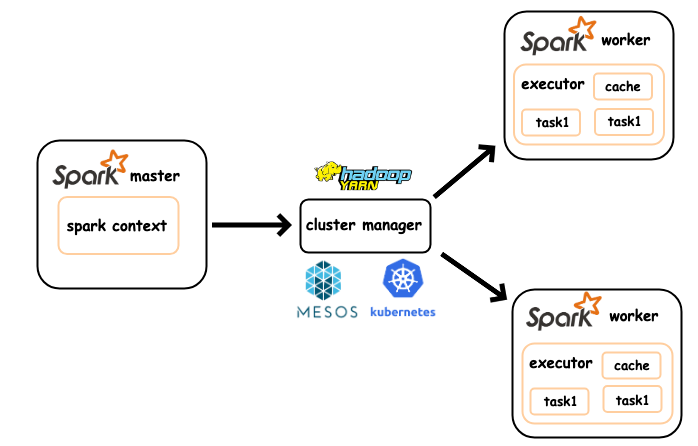
Like Hadoop, Spark follows a simple master and worker architecture. A machine is dedicated to manage the Spark cluster, which is known as the Spark Master node (c.f. namenode in a Hadoop Cluster). A set of machines are in charge of running the actual computation, namely, the Spark Worker nodes (c.f. data nodes in a Hadoop Cluster).

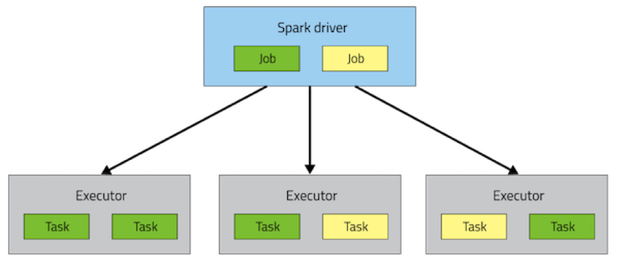
A driver is a program that runs on the Spark Master node, which manages the interaction between the application and the client. Upon a job submission from the client, a Spark driver schedules the jobs by analyzing the sub tasks dependency and allocate the sub tasks to the executors. A list of executors (runnning on some worker nodes) receive tasks from the driver and reports the result upon completion.

Spark Task Scheduling¶

In this section, we take a look at how Spark divides a given job into tasks and schedules the tasks to the workers.

As illustrated by the above diagram Spark takes 4 stages to schedule the job.

1. Given a job, Spark builds a directed acyclic graph (DAG) which represents the dependencies among the operations performed in the job.
2. Given the DAG, Spark splits the graph into multiple stages of tasks.
3. Tasks are scheduled according to their stages, A later stage must not be started until the earlier stages are completed.
4. Tasks scheduled to the workers then executed.

A simple example¶

Let's consider a simple example

1
2
3

# spark job 1
r1 = sc.textFile("...")
r2 = r1.map(f) 

graph TD
    r1 --map--> r2 

It is clear that there is only one stage, (because there is only one operation, one set of inputs and one set of outputs).

The Task Scheduler allocate the tasks in parallel, as follows.

A less simple example¶

Let's consider another example

1
2
3
4
5
6
7
8
9

# spark job 2
r1 = sc.textFile("...")
r2 = r1.map(f)
r3 = sc.textFile("...")
r4 = r3.map(g)
r5 = r2.join(r4)
r6 = r5.groupByKey()
r7 = r6.map(h)
r8 = r7.reduce(i)

The DAG is as follows

graph TD;
r1 --map--> r2 
r3 --map--> r4
r2 --join--> r5
r4 --join--> r5
r5 --groupByKey--> r6
r6 --map--> r7
r7 --reduce--> r8

There are mulitple way of dividing the above DAG into stages. For instance, we could naively turns each operation (each arrow) into a stage (we end up with many stages and poor parallelization) or we group the simple paths (straight line paths) into a stage.

Spark takes a more intelligent approach by classifying different types of dependencies.

• Narrow dependencies - Input partition used by at most 1 output partition

• Wide dependencies - Input partition used by more than one output partitions

Thus for Spark Job 2, we further annotate the DAG with dependency types.

graph TD;
r1 --map/narrow--> r2 
r3 --map/narrow--> r4
r2 --join/narrow--> r5
r4 --join/wide--> r5
r5 --groupByKey/wide--> r6
r6 --map/narrow--> r7
r7 --reduce--> r8

All the map operations are narrow. The join of r2 and r4 should be wide. However since the result must be ordered either by r2's partition order or r4's. Only one side of the operation is wide. In this case, we assume r5's partition follows r2's, hence r2 to r5 is narrow. groupByKey operations are wide.

Next we can decide how many stages we need by

1. allowing narrow dependencies preceding the same wide dependency to the grouped under the same stage, because they do not incur any network I/O.
   • We apply task parallelism here.,
2. wide dependency initiates a new stage, as we need to wait for all the data operands to be fully computed before the operation being executed.

graph TD;
r1 --map/narrow/1--> r2 
r3 --map/narrow/1--> r4
r2 --join/narrow/2--> r5
r4 --join/wide/2--> r5
r5 --groupByKey/wide/3--> r6
r6 --map/narrow/3--> r7
r7 --reduce/3--> r8

In the above, we stage the first two map operations. The join operation is assigned to the 2^nd stage. The groupByKey initiates the 3^rd stage which includes the following map and reduce.

Spark performance tuning¶

Knowing how Spark schedules a job into stages of sub tasks. We can optimize the job by rewriting it into an equivalent one such that

• Pre-partition or re-partition of the data
• Cache the common intermediate data

Pre-partition or re-partition of the data¶

Recall that a spark job is represented a DAG of stages

If we know the join operation and pre- (or re-) arrange the data according to the key to partition mapping, we could reduce the shuffling.

1
2
3
4

d1 = [(1, "A"), (2, "B"), (1, "C"), (2, "D"), (1, "E"), (3, "F")]
d2 = [(1, 0.1), (2, 0.2), (2, 3.1), (3, 0)]
r1 = sc.parallelize(d1) 
r2 = sc.parallelize(d2)

let assume that r1 is by default partitioned randomly into two partitions and so is r2.

1
2
3
4
5
6
7
8

r1.glom().collect() # collect rdd into list by retaining the partition
r2.glom().collect()
# r1 being partitioned 
[[(1, 'A'), (2, 'B'), (1, 'C')],   # p1
  [(2, 'D'), (1, 'E'), (3, 'F')]]  # p2
# r2 being partitioned
[[(1, 0.1), (2, 0.2)],  # p3
  [(2, 3.1), (3, 0)]])  # p4

next we would like join r1 with r2 by key, i.e. the first component of the pairs

1
2

r3 = r1.join(r2)
r3.glom().collect()

the result will be stored in three partitions

1
2
3

[[(1, ('A', 0.1)), (1, ('C', 0.1)), (1, ('E', 0.1))], # p1
 [(2, ('B', 0.2)), (2, ('B', 3.1)), (2, ('D', 0.2)), (2, ('D', 3.1))], # p2
 [(3, ('F', 0))]] # p3

Note that the actual order of the collected result might not be same as above, Spark tries to reuse partitions being created whenever possible. (For breivity we omit an empty partition p4.)

As observed, there are tuple transferred from p1 to p2, e.g. (2, 'B') and from p2 to p1, e.g. (1, 'E'). These transfers can be eliminited if we manually control the partitioning of the initial RDDs,

1
2
3
4

r4 = sc.parallelize(d1).partitionBy(3, lambda key: key)
r5 = sc.parallelize(d2).partitionBy(3, lambda key: key)
r4.glom().collect()
r5.glom().collect()

1
2
3
4
5
6
7
8

# r4 is partitioned 
[[(3, 'F')], #p1 
 [(1, 'A'), (1, 'C'), (1, 'E')], #p2 
 [(2, 'B'), (2, 'D')]] #p3
# r5 is partitioned 
[[(3, 0)],  #p4
[(1, 0.1)], #p5
[(2, 0.2), (2, 3.1)]] #p6

when we perform the join

1
2

r6 = r4.join(r5)
r6.glom().collect()

we have

1
2
3
4
5

[
[(3, ('F', 0))], #p1
[(1, ('A', 0.1)), (1, ('C', 0.1)), (1, ('E', 0.1))], #p2
[(2, ('B', 0.2)), (2, ('B', 3.1)), (2, ('D', 0.2)), (2, ('D', 3.1))] #p3
]

• Sample code can be found here.

  1	https://colab.research.google.com/drive/1XO1hqcRCn9JKu0tkRb0ANQylCnBod3B-?usp=sharing

Cache the intermediate data¶

Recall that in Spark transformation are lazy until a shuffling is required. Laziness is a double-edged sword.

In the above, the orange partition (data) is being used by 3 different "sinks". If all the operations above the last levels are transformations (i.e. lazy.) Having 3 sink operations will require most of the intermediate partitions (all boxes except for the last)

For example consider the following

1
2
3
4
5
6
7
8

data = [(1, 100), (1, 90), (1, 80), (2, 80), (2, 30), (2, 50)]
r1 = sc.parallelize(data)
r2 = r1.map( lambda x:(x[0], x[1] * 0.01))
r3 = r2.groupByKey()
r4 = r3.map( lambda x:(x[0], std(x[1])))
r5 = r3.map( lambda x:(x[0], min(x[1])))
r4.collect()
r5.collect()

There are two downstream operation of r3, namely r4 computing the standard deviation by key, and r5 computing the minimum by key.

Due to the fact that r3 is lazy. The r4.collect() action (sink) triggers the computation of r1 to r3 and r4. The r5.collect() triggers the recomputation of r1 to r3 and the computation of r5.

If we materialize r3 and cache it, we would avoid the recomputation of r1 to r3.

1
2
3
4
5
6
7
8

data = [(1, 100), (1, 90), (1, 80), (2, 80), (2, 30), (2, 50)]
r1 = sc.parallelize(data)
r2 = r1.map( lambda x:(x[0], x[1] * 0.01))
r3 = r2.groupByKey().cache()
r4 = r3.map( lambda x:(x[0], std(x[1])))
r5 = r3.map( lambda x:(x[0], min(x[1])))
r4.collect()
r5.collect()

• Sample code

  1	https://colab.research.google.com/drive/1QqUSa5Kkjpw3Avw2DlWX9ZMrZcsnDz5x?usp=sharing

Other optimization tricks¶

Besides the above mentioned two approaches, a trick that we've used in RDBMS for optimization is also applicable to Spark. i.e. apply filter as early as possible so as to reduce the size of intermediate output.

Another Spark specific optimization trick is to rewriting groupByKey().map(...) by reduceByKey(...). However in some cases, a rewrite solution might not exist.

Spark Failure Recovery¶

Recall that for any MapReduce implementation to produce deterministic results. The computation must be pure.

It turns out that purity property makes failure recovery much easier. For each Spark job, a lineage of the sub tasks is computed. In the event of failure, the Spark driver will refer to the lineage and recompute the affected sub-tasks. Thanks to the purity property, partially completed and incomplete computation can always be computed without the need of restoring the original state.

For instance consider the following job

Where all the square boxes denote the partitions of some RDDs, suppose partition C1 is faulty.

Based on the diagram (lineage), we know that we can recompute C1 elsewhere by using B1 and B2.

Spark DataFrame¶

Besides Spark RDD, Spark offers DataFrame as a higher level API interface to the programmers and data engineers. The ussage is influenced and inspired by Python's Pandas.

In a nutshell, a dataframe can be seenas a schema plus a set of RDDs.

Since Dataframe was designed for machine learning applications, it adopts the column-based data structure instead of row based.

Question: Why Columnar?¶

Hint: How data are used in ML model?

Creating Spark Dataframe¶

We can convert a Spark rdd into a dataframe.

1
2
3

data = [(1, 100), (1, 90), (1, 80), (2, 80), (2, 30), (2, 50)]
r1 = sc.parallelize(data)
df1 = r1.toDF("id", "score")

Alternatively, we can create DataFrames directly from a CSV file.

Given file hdfs://127.0.0.1:9000/foo.csv

1
2
3
4
5

foo,bar
1,true
2,false
3,true
4,false

1
2
3
4
5

df = sparkSession.read\
     .option("header", "true")\
     .option("inferSchema", "true")\
     .csv("hdfs://127.0.0.1:9000/foo.csv")
df.printSchema()

1
2
3

root
 |-- foo: integer (nullable = true)
 |-- bar: boolean (nullable = true)

Note in the above, Spark loads a text file (CSV) from HDFS and infers the schema based on the first line and the values.

DataFrame APIs¶

Let's have tour of the Spark DataFrame APIs by going through some examples.

Here is the data we use in the examples

1
2
3
4
5
6
7

data = [("100001", "Ace", "50043", 90), \
        ("100002", "Brandon", "50043", 95), \
        ("100003", "Cheryl", "50043", 80)]
distData = sc.parallelize(data)
df = distData.toDF(["studentid", "name", \
                 "module", "score"])
df.show()

Column Projection¶

To project (select the columns) we use the .select() method.

1
2
3
4

df.select(df["studentid"], df["score"]).show() # or

from pyspark.sql.functions import col
df.select(col("studentid"), col("score")).show() 

To compute a new column based on the existing one, we use an overloaded version of the .select() method whose first argument is the operation and the second argument is the name of the new column.

1
2
3
4

from pyspark.sql.functions import concat, lit
df.select(concat(df["studentid"]\
         ,lit("@mymail.sutd.edu.sg"))\
   .alias("email")).show()

For the full set of builtin funtcions for column operations.

1

https://spark.apache.org/docs/3.0.1/api/python/pyspark.sql.html

There are times we want to create a new column and keeping the old columns.

1
2
3

df.withColumn("email",concat(col("studentid"),\
   lit("@mymail.sutd.edu.sg")))\
   .show()

Row filtering¶

For row filterings, we use .filter() method.

1

df.filter(col("studentid") == "100003").show()

And similar for range filter

1

df.filter(col("score") > 90).show()

lit() is optional here, pyspark inserts it for us.

Group By and Aggregation¶

For aggregation, we use .groupBy()

1

df.groupBy("module").avg().show()

Join¶

For join, we use .join()

1
2
3
4
5
6
7

moddata = [("50043", "Database and Big Data Systems")]
distmodData = sc.parallelize(moddata)
moddf = distmodData.toDF(["module", "modname"])

df.join(moddf, df["module"] == moddf["module"], "inner")\
   .select(df["studentid"], df["name"], df["module"],\
   df["score"], moddf["modname"]).show()

Spark SQL¶

Besides Spark RDD, Spark allows program to use SQL query to perform data transformation and action.

For example,

1
2

df.createOrReplaceTempView("students")
spark.sql("SELECT * FROM students").show()

With some notebook support, we can even use SQL to perform data visualization.

Spark Machine Learning¶

Spark comes with two differen Machine Learning libraries.

• MLLib package - for RDD
• ML package - for dataframe (and dataset)

MLLib package¶

MLLib package offers a lower level access of data type such as vectors and label points.

Vectors¶

In Spark, vectors are local data collection (non-distributed). There are dense vectors and sparse vectors.

• For dense vector - all values need to be specified when it is created

  1 2	from pyspark.mllib.linalg import * dv = Vectors.dense(1.0, 0.0, 3.0)

• For sparse vector - we don't need to specify all the value, instead we specify the size of the vector as well as the non-zero values.

1
2

sv1 = Vectors.sparse(3, [0, 2], [1.0, 3.0]) # or
sv2 = Vectors.sparse(3, [(0, 1.0), (2, 3.0)])

Labeled points¶

With features extracted as vectors. We need to find a way to label them.

Spark MLLib comes with its own labeled point data type

1
2
3
4
5
6
7
8

from pyspark.mllib.regression import *
# Create a labeled point with a positive label
# and a dense feature vector.
pos = LabeledPoint(1.0, Vectors.dense(1.0, 0.0, 3.0))
# Create a labeled point with a negative label
# and a sparse feature vector.
neg = LabeledPoint(0.0, Vectors.sparse(3, \
      [(0, 1.0), (2, 3.0)]))

Training an inference¶

With labeled points defined and extracted, assuming

1
2

pos = ... # RDD of labeled points
neg = ... # RDD of labeled points

we train the model

1
2
3
4

from pyspark.mllib.classification import SVMWithSGD
training = pos + neg
numIteration = 20
model = SVMWithSGD.train(training, numIterations)

which is a support vector machine with SGD algorithm.

To perform inference, we need to feed a new sample as a vector to the model.

1
2

newInstance = Vectors.dense(1.0, 2.0, 3.0)
model.predict(newInstance)

ML Package¶

As the ML package is targetting the higher level data structures (Dataframe and Dataset), machine learning models in ML package are built using the pipeline.

The Training Pipeline¶

One of the training pipelines is known as the estimator

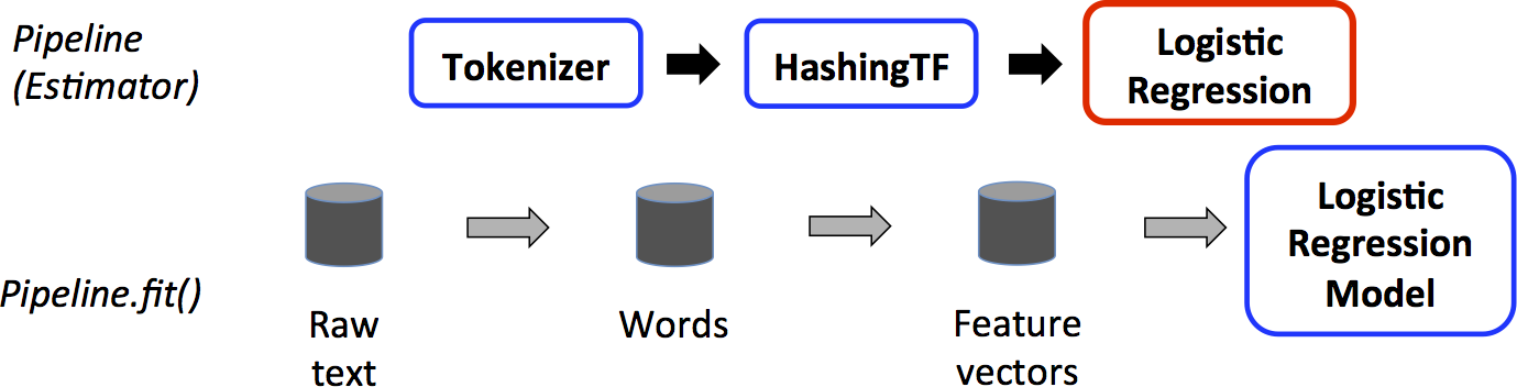
In the diagram above, it illustrate the pipeline of training a classifier using logistic regression.

 1
 2
 3
 4
 5
 6
 7
 8
 9
10
11
12
13
14
15
16
17
18
19
20
21

from pyspark.ml import Pipeline, PipelineModel
from pyspark.ml.classification import LogisticRegression
from pyspark.ml.feature import HashingTF, Tokenizer
data = spark.createDataFrame([
    (0, "a b c d e spark", 1.0),
    (1, "b d", 0.0),
    (2, "spark f g h", 1.0),
    (3, "hadoop mapreduce", 0.0),
    (4, "spark is scaling", 1.0),
    (5, "random stuff", 0.0)
], ["id", "text", "label"])

train, test = data.randomSplit([0.7, 0.3], seed=12345)
# Configure an estimator pipeline, 
tokenizer = Tokenizer(inputCol="text", outputCol="words")
hashingTF = HashingTF(inputCol=tokenizer.getOutputCol(), outputCol="features")
lr = LogisticRegression(maxIter=10, regParam=0.001)
pipeline = Pipeline(stages=[tokenizer, hashingTF, lr])

# Fit the pipeline to train
model = pipeline.fit(train)

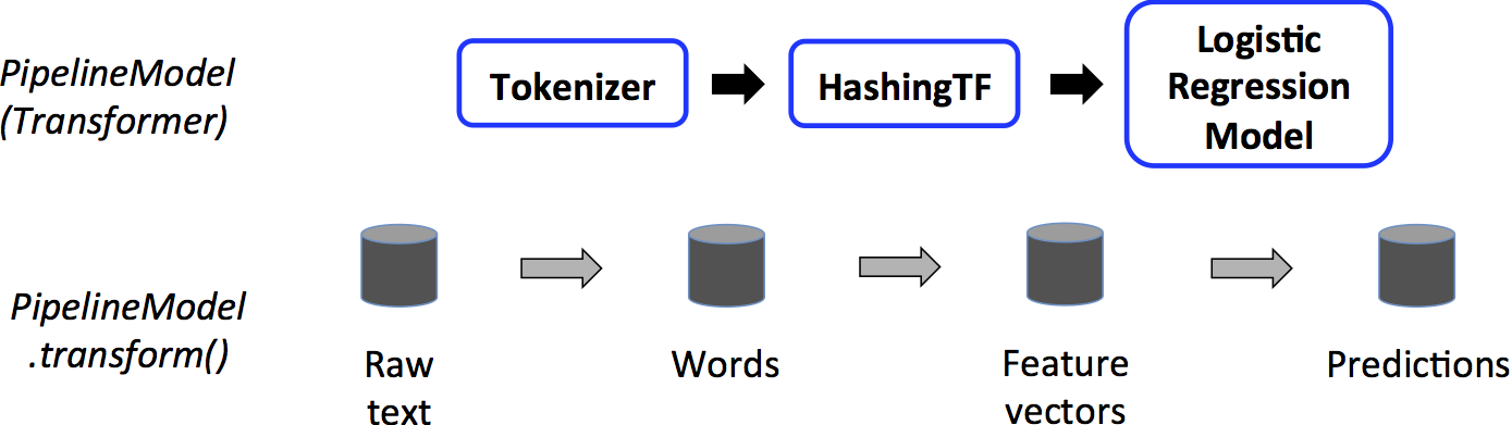
The transformer pipeline¶

The inference pipeline on the other hand is known as the transformer

1
2
3
4
5
6

# Configure an Inference pipeline
# Note now model include tokenizterm hashingTF, and lr
pipeline_model = PipelineModel(stages=[model]) 
prediction = pipeline_model.transform(test)
result = prediction.select("id", "text", "probability", "prediction")
result.show()

Sample code¶

1

https://colab.research.google.com/drive/1ZI-BG2XaB3AOyzPrXeqO7xqNGYycCJ-U?usp=sharing

Spark Streaming¶

Spark offers Streaming API which handles real time (infinite) input data.

The real-timeness is approxmiated by chopping the data stream into small batches. These small batches are fed to the spark application.

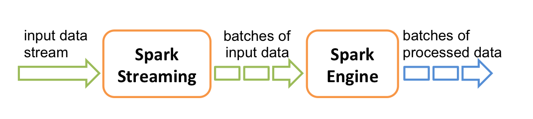
For example the following is a simplified version of a data streaming application that computes the page views by URL over time.

1
2
3
4
5
6
7
8
9

from pyspark import SparkContext
from pyspark.streaming import StreamingContext
sc = SparkContext("local[2]", "PageView")
ssc = StreamingContext(sc, 1)

lines = ssc.socketTextStream("localhost", 9999)
pageViews = lines.map(lambda l:parse(l))
ones = pageViews.map(lambda x: (x.url, 1))
counts = ones.runningReduce(lambda x,y: x+y)

Additional References¶

• Spark Dataframe
• https://spark.apache.org/docs/latest/sql-getting-started.html
• Spark MLLib and ML package
• https://spark.apache.org/docs/latest/ml-guide.html
• Spark Streaming
• https://spark.apache.org/docs/latest/streaming-programming-guide.html